|
Number of Branches: Checking plausibility
 LIB "primdec.lib";


           ring r=0,(x,y,z),ds;

           ideal i=x^4-y*z^2,x*y-z^3,y^2-x^3*z;

           qhweight(i);
The isolated space curve singularity is quasihomogeneous.
           resolution ires=mres(i,0);

           ires;
|
==>
|
        1       3       2
      rr <--  rr <--  rr

      0       1       2
|
It is of Cohen-Macaulay type t=2.
LIB "sing.lib";
T_1(i);
|
==>
|
// dim T_1 = 13
_[1]=gen(6)+2z*gen(5)
_[2]=gen(4)+3x2*gen(2)
_[3]=gen(3)+gen(1)
_[4]=x*gen(5)-y*gen(2)-z*gen(1)
_[5]=x*gen(1)-z2*gen(2)
_[6]=y*gen(5)+3x2z*gen(2)
_[7]=y*gen(2)-z*gen(1)
_[8]=2y*gen(1)-z2*gen(5)
_[9]=z2*gen(5)
_[10]=z2*gen(1)
_[11]=x3*gen(2)
_[12]=x2z2*gen(2)
_[13]=xz3*gen(2)
_[14]=z4*gen(2)
|
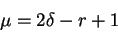
The Tjurina number is 13. As the quasihomogeneous space curve singularity is
Cohen-Macaulay of codimension 2, it is unobstructed and hence we can apply the
formula

|
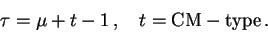
Hence the Milnor number is 12, in particular it is
even. By the formula
this contradicts the number of branches (= 2) we computed
before. |
==> We have to decompose the second component further, e.g. using
normalization.
<-- Branches of an isolated space curve singularity
<-- computed via Primary Decomposition
--> computed via Normalization
--> computed via Factorizing Gröbner
|