|
|
C.6.2.1 The algorithm of Conti and Traverso
The algorithm of Conti and Traverso (see [CoTr91])
computes  via the
extended matrix via the
extended matrix  ,
where ,
where  is the is the  unity matrix. A lattice basis of unity matrix. A lattice basis of  is
given by the set of vectors is
given by the set of vectors
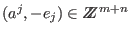 , where , where  is the
  -th row of -th row of  and and  the -th coordinate vector. We
look at the ideal in the -th coordinate vector. We
look at the ideal in
![$K[y_1,\ldots,y_m,x_1,\ldots,x_n]$](sing_720.png) corresponding to
these vectors, namely corresponding to
these vectors, namely
We introduce a further variable  and adjoin the binomial and adjoin the binomial
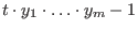 to the generating set of to the generating set of  , obtaining
an ideal , obtaining
an ideal  in the polynomial ring in the polynomial ring
![$K[t,
y_1,\ldots,y_m,x_1,\ldots,x_n]$](sing_725.png) . is saturated w.r.t. all
variables because all variables are invertible modulo . Now
can be computed from by eliminating the variables . is saturated w.r.t. all
variables because all variables are invertible modulo . Now
can be computed from by eliminating the variables
 . .
Because of the big number of auxiliary variables needed to compute a
toric ideal, this algorithm is rather slow in practice. However, it has
a special importance in the application to integer programming
(see Integer programming).
|
 Online Manual


